In the rapidly evolving fields of machine learning (ML) and deep learning, neural networks have emerged as the backbone of cutting-edge applications. From natural language processing to computer vision, deep neural networks are used in virtually every AI-driven technology today. One aspect that is often overlooked, yet critical to network performance, is weight initialization—the method used to set the starting values of a neural network’s weights before training begins.
Proper initialization can make the difference between a model that converges quickly to an accurate solution and one that never trains properly. Conversely, poor initialization can lead to issues like slow convergence, vanishing or exploding gradients, or trapped local minima. In this article, we will explore best practices for neural network initialization, discuss the underlying principles, and provide actionable guidance for practitioners in both ML and deep learning.
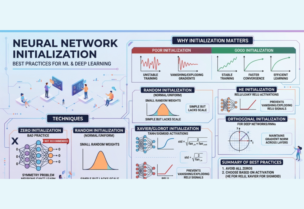
Why Initialization Is Critical in Neural Networks
At its core, a neural network is a function composed of layers of interconnected neurons. Each neuron applies a weighted transformation to its inputs and passes it through an activation function. These weights and biases are initially unknown and must be set before training. This is where initialization plays a crucial role.
Key Problems Caused by Poor Initialization
-
Vanishing Gradients:
In deep networks, gradients may shrink as they backpropagate through many layers, especially with sigmoid or tanh activations. When gradients vanish, learning slows dramatically or stops altogether. -
Exploding Gradients:
Large initial weights can cause gradients to grow exponentially, leading to unstable updates and divergence during training. -
Slow Convergence:
If weights are not properly scaled, the network may require many more epochs to reach a reasonable solution, increasing computation time and resource usage. -
Symmetry Problem:
If all neurons in a layer are initialized identically, they will learn the same features, reducing the representational power of the network. Randomization is essential to break this symmetry.
Effective initialization sets the network on a favorable path from the beginning, enabling faster convergence and higher accuracy.
Common Initialization Techniques
Over the years, several initialization methods have been developed to address the challenges above. Choosing the right method depends on network depth, activation functions, and layer types.
1. Zero Initialization
Zero initialization sets all weights to zero. While it may seem intuitive, it is generally unsuitable for hidden layers due to the symmetry problem. If all weights are identical, neurons in the same layer will perform identical computations and learn the same features, making the network ineffective. Biases, however, can safely be initialized to zero.
Use Case:
-
Biases in hidden layers
-
Not recommended for weights
2. Random Initialization
Random initialization assigns small random values to weights, often sampled from uniform or normal distributions. This breaks symmetry and allows neurons to learn different features. However, the variance of the distribution must be carefully controlled. Too large a range leads to exploding gradients, while too small a range can cause vanishing gradients.
Use Case:
-
Shallow networks
-
Simpler ML models without deep layers
3. Xavier/Glorot Initialization
Proposed by Glorot and Bengio, Xavier initialization (also called Glorot initialization) is designed for networks with sigmoid or tanh activation functions. It scales the weights based on the number of input and output neurons:
W∼U(−6nin+nout,6nin+nout)W sim mathcal{U}Big(-sqrt{frac{6}{n_{in} + n_{out}}}, sqrt{frac{6}{n_{in} + n_{out}}}Big)W∼U(−nin+nout6,nin+nout6)
Here, ninn_{in}nin and noutn_{out}nout are the number of neurons in the input and output layers of a given layer. Xavier initialization keeps the variance of activations consistent across layers, helping prevent vanishing or exploding gradients.
Use Case:
-
Deep networks with sigmoid or tanh activations
-
Feedforward networks
4. He/Kaiming Initialization
He initialization or Kaiming initialization is optimized for networks using ReLU (Rectified Linear Unit) and its variants. Since ReLU outputs zero for half of the inputs, the variance of weights needs to be adjusted to maintain stable activation across layers:
W∼N(0,2nin)W sim mathcal{N}Big(0, frac{2}{n_{in}}Big)W∼N(0,nin2)
This method prevents dead neurons and improves training stability for deep networks with ReLU activations.
Use Case:
-
Deep networks with ReLU, Leaky ReLU, or ELU activations
-
Convolutional neural networks (CNNs)
5. Orthogonal Initialization
Orthogonal initialization involves setting weights to an orthogonal matrix, preserving the variance of signals throughout the network. It is particularly useful for deep feedforward networks and recurrent neural networks (RNNs), where long-term dependencies make training more sensitive to initialization.
Use Case:
-
RNNs
-
Deep feedforward networks
6. Layer-Specific Initialization
Modern architectures often benefit from layer-specific initialization. Different layers may require different initialization strategies:
-
Convolutional Layers: He initialization for ReLU activations
-
Batch Normalization Layers: Scale initialized to 1, bias to 0
-
Embedding Layers: Small random values sampled from a normal distribution
Tailoring initialization to layer type improves learning efficiency and stability.
Best Practices for Neural Network Initialization
-
Match Activation Functions: Use Xavier for sigmoid/tanh, He for ReLU/Leaky ReLU.
-
Avoid Large Initial Weights: Prevents exploding gradients.
-
Monitor Training Early: Check for vanishing or exploding gradients and adjust initialization if necessary.
-
Combine with Batch Normalization: Stabilizes activation distributions and reduces sensitivity to initialization.
-
Bias Initialization: Often set to zero or small positive values for ReLU layers to improve early learning.
-
Use Library Defaults: Frameworks like TensorFlow and PyTorch have robust default initializations, reducing trial-and-error.
-
Test Multiple Strategies: For complex networks, experimenting with different initializations can improve performance.
Practical Examples in Deep Learning
-
CNNs for Image Recognition: He initialization ensures stable gradients in convolutional layers using ReLU.
-
RNNs for Sequence Modeling: Orthogonal initialization stabilizes long-term dependencies in LSTM or GRU networks.
-
Multi-Layer Perceptrons (MLPs): Xavier initialization balances signal variance across hidden layers using tanh or sigmoid activations.
By following these best practices, practitioners can prevent common pitfalls and accelerate training without sacrificing model accuracy.
Initialization in ML vs Deep Learning
Traditional ML algorithms like linear regression, logistic regression, decision trees, and SVMs do not rely on weight initialization. In contrast, deep learning models, due to their depth, non-linear activations, and gradient-based optimization, are highly sensitive to initialization. Poor initialization in deep networks can prevent convergence entirely, whereas shallow networks are more forgiving.
Conclusion
Neural network initialization is a foundational aspect of deep learning that significantly impacts training speed, convergence stability, and final model performance. Using the right initialization methods—tailored to network architecture and activation functions—can prevent vanishing or exploding gradients, improve convergence, and enhance overall model performance.
Key Takeaways:
-
Always match initialization to the activation function (Xavier for sigmoid/tanh, He for ReLU).
-
Avoid symmetric or zero weights in hidden layers to prevent neurons from learning identical features.
-
Consider layer-specific initialization for complex architectures.
-
Use modern deep learning frameworks’ defaults as a reliable starting point.
-
Monitor early training behavior to adjust initialization if needed.
By adhering to these best practices, developers can ensure that their neural networks start from a solid foundation, ultimately leading to stable, efficient, and high-performing machine learning and deep learning models.